Let's consider an improved version of the function VLOOKUP - VLOOKUP3, which gives us the opportunity to substitute values when two conditions match. This function can be useful in cases where we do not have unique values in the field on which we need to perform a combination.
Suppose we need to join two tables, but we have no unique values:
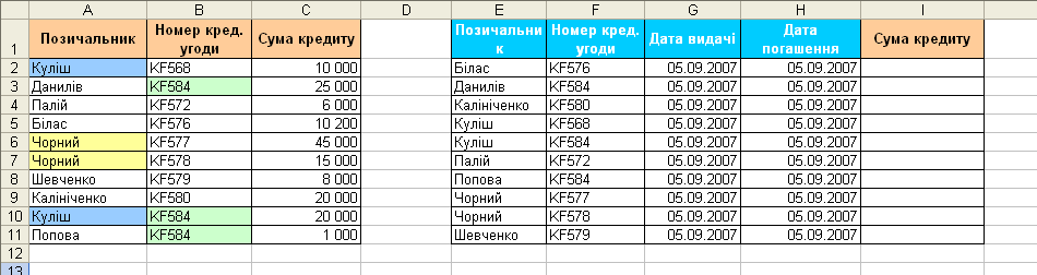
As you can see, we have borrowers with the same surnames and credit agreements with the same numbers. Combine with a normal function VLOOKUP will be problematic because it matches only one condition at a time and only the first value found.
Let's redo our usual VLOOKUP for substituting values according to two conditions.
Open the menu Service - Macro - Editor Visual Basic , insert the new module (menu Insert - Module ) and copy the text of this one there functions:
Function VLOOKUP3(Table1       As Range, _
                  SearchValue1 As Variant, _
                  Table2       As Range, _
                  SearchValue2 As Variant,_
				  ResultColumn As Range)
  'moonexcel.com.ua
  Dim i As Integer

  For i = 1 To Table1.Rows.Count
    If Table1.Cells(i, 1) = SearchValue1 Then
      If Table2.Cells(i, 1) = SearchValue2 Then
        VLOOKUP3 = ResultColumn.Cells(i, 1)
        Exit For
      End If
    End If
  Next i

End Function
Close the editor Visual Basic and return to Excel.
Now in Function Wizards in the category User defined you can find our VLOOKUP3 function and use it. The syntax of the function is as follows:
=VLOOKUP3( range1 ; searched_value1 ; range2 ; searched_value2 ; the range from which we substitute values )
That is, in order to correctly substitute the loan amount by last name and agreement number in the cell E15 you will need to enter:
=VLOOKUP3($A$2:$A$11; A15; $B$2:$B$11; B15; $C$2:$C$11)
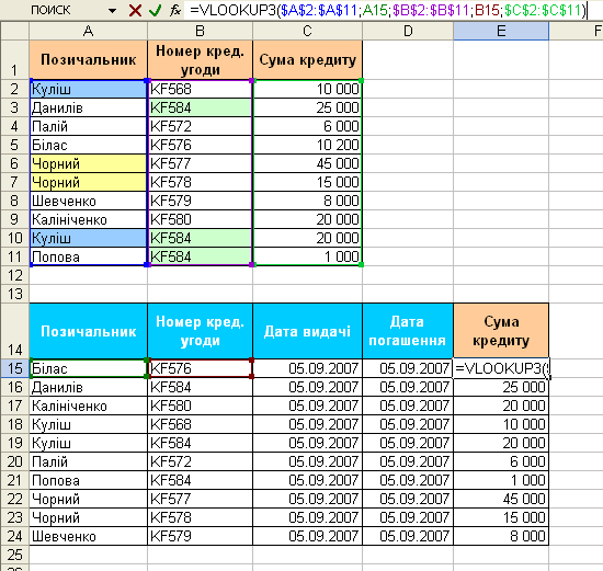
Also, do not forget to fix the ranges with a dollar sign ($) , so that we do not miss the ranges when copying the formula (for quick fixing, you can also use the F4 key).

