DAX-Lesson 3. Data selection function FILTER

Description

In this article, we will look at another important function, which is called FILTER and is used in conjunction with the CALCULATE function. This function does the same thing as we do when we try to filter the data in the table by the values in a certain column. That is, in other words, this function reduces the size of the table with which, in turn, the CALCULATE function will work.

Syntax of function FILTER()

=FILTER(< table >, < filter >)

< table >

The table we want to filter. Also, there can be an expression that returns a table as a result:

1. 'TableName'
2. ALL( 'TableName' ) or ALL( 'TableName' [ Column name ])
3. FILTER( 'TableName' , 'TableName' [ Column name ] = " Green ")
4. VALUES( 'TableName' [ Column name ])

< filter >

A comparison expression that is executed for each row of the table. Here are the conditions for selecting values:

1. [ Column name ] = Auto
2. [ Column name ] >= 6

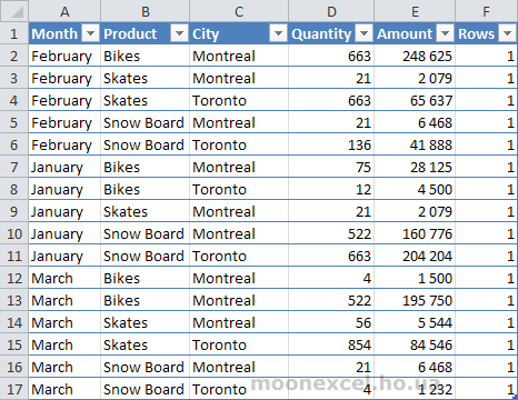
Let's see how it looks in practice. Suppose we have such a table, which is called Demo :

We need to count the number of records for a product Bikes (bicycles) and display the result in a summary table. For this, we will write down the following formula:

=CALCULATE(COUNTROWS(Demo); FILTER(Demo; Demo[Product]="Bikes"))

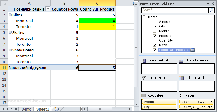
As a result, we will get the following values in the Count_All_Product field:

What did the FILTER function do? It reduced the size of the table, as we do in Excel by setting a filter in the column Product and filtering only records with values Bikes :

Then she counted the number of all rows in the reduced table. We see that there are no entries in the Count_All_Product field in the other rows, because there are no skates in the new table (Skates) and snowboards (Snow Board) .