The built-in function VLOOKUP is one of the most powerful functions in Excel. But it has one significant drawback - it finds only the first occurrence of the desired value in the table and only in the far right column. But if you need the 2nd, 3rd and not the last one?
Let's say we have a table of processed loans like this:
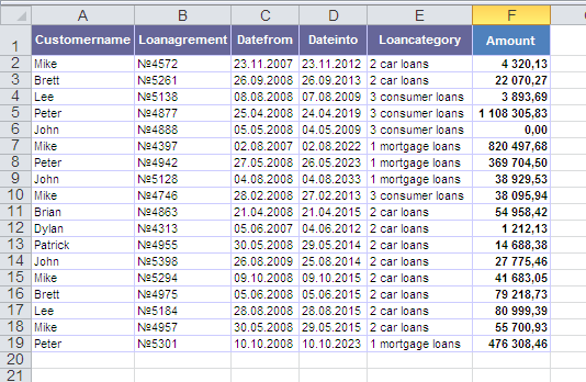
We need to know, for example, what was the amount of the third loan issued to Mike or when John executed his second agreement. Built-in function VLOOKUP knows how to search only the first occurrence of a name in the table and will not help us.
Let's write our function, which will search not only the first, but also any subsequent (Nth) occurrence. Let's call it, for example, VLOOKUP2.
Open the menu Service - Macro - Editor Visual Basic , insert the new module (menu Insert - Module ) and copy the text of this function there:
Function VLOOKUP2(Table           As Range, _
                  SearchColumnNum As Integer, _
                  SearchValue     As Variant, _
                  N               As Integer, _
                  ResultColumnNum As Integer)
  'moonexcel.com.ua
  Dim i      As Integer
  Dim iCount As Integer

  For i = 1 To Table.Rows.Count
    If Table.Cells(i, SearchColumnNum) = SearchValue Then
      iCount = iCount + 1
    End If
    If iCount = N Then
      VLOOKUP2 = Table.Cells(i, ResultColumnNum)
      Exit For
    End If
  Next i
End Function
Close the editor Visual Basic and return to Excel.
Now in Function Wizards in the category User defined you can find our VLOOKUP2 function and use it. The syntax of the function is as follows:
=VLOOKUP2( table ; column_number_where_we_search ; searched_value; entry_number ; column_number_from_which_we_take_the_value )
That is, in order to find the amount of the third loan issued to Mike, you will need to enter:
=VLOOKUP2(A2:A19; 1; "Mike"; 3; 4)

