Let's consider how to quickly combine two large tables together with columns and rows, that is, make a selection not by one parameter (as the functions VLOOKUP or HLOOKUP), but by two at once (using the functions INDEX and MATCH).
If you are familiar with the function VLOOKUP or its horizontal analogue HLOOKUP, then you should remember that these wonderful functions look for information by only one parameter, that is, in a one-dimensional array - by row or by column. And if we need to select data from a two-dimensional table by the coincidence of two parameters at once - both row and column at the same time? Let's consider several options for combining tables.
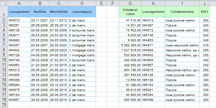
Suppose we need to combine two tables that display the loan portfolio and the collateral portfolio:

We can start using the VLOOKUP function to combine each individual column, but if our tables have an extremely large number of rows and columns, this exercise can turn into a real pain. However, there is a rather simple way out of this situation, since Excel has two excellent functions, INDEX and MATCH from the category References and arrays
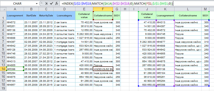
Okay, so what do we need to do to quickly join the two tables? Let's start by copying the header of the second table (the one we will join) and paste it next to the header of the first table. By the name of the cap, the function MATCH will give us the serial number of the column, and according to the transaction number - the serial number of the line we need.
In fact, we want to find the value of a cell from the intersection of a particular row and column in a table. For clarity, let's divide the task into three stages:
So, combining all of the above into one formula, we get for the cell F14 the following formula:
=INDEX(J2:M18; MATCH(A14; K2:K18; 0); MATCH(F1; J1:M1; 0))

That way, by stretching our formula over the entire range, we'll correctly attach the extra fields. You also need to pay attention that when stretching the formula, we need to fix the ranges with a dollar sign ($) (for fixing, you can use the F4 key), for searching by cap, fix only the line ( F$1 ), for searching by transaction numbers - only column ( $A14 ).
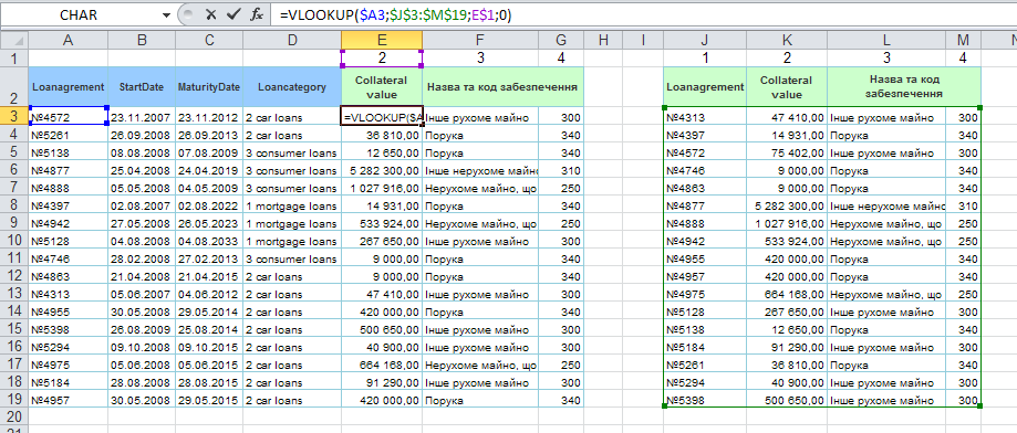
Let's slightly modify the previous example and suppose that we have similar tables, but their headers are combined, so the MATCH function will not help us to correctly determine the serial number of the column.
In this case, we can create a technical field above the table, and insert column numbers manually. Then, we can use the already familiar VLOOKUP function.

So, the formula for our second option will be as follows:
=VLOOKUP($A3; $J$3:$M$19; E$1; 0)
Again, don't forget to mark the range and corresponding search fields with a sign $ , so that the formula works correctly and does not give an error when shifting the ranges.