VlookupSeq function (VLOOKUP2) for LO Calc

VLOOKUPSEQ() Description

The built-in function VLOOKUP is one of the most powerful functions in LO Calc . But it has one significant drawback - it finds only the first occurrence of the desired value in the table and only in the far right column. But if you need the 2nd, 3rd and not the last one?

The modified VLOOKUPSEQ function can return any match (not just the first one found) from any specified column.

Main Features of the VLOOKUPSEQ Function

Syntax:

=VLOOKUPSEQ(LookupValue; LookupArray; ReturnArray; Seq)

Parameters:

• LookupValue: The meaning we are looking for.
• LookupArray: The column in which we are searching.
• ReturnArray: The column from which we return the associated value.
• Seq: The sequence number of the match found.

Example Usage

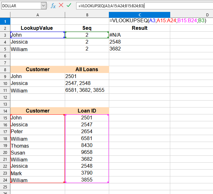
The VLOOKUPSEQ() function is easy to use. You just need to specify the search range and the column from which the values will be taken, as well as the sequence number of the required match and LO Calc will automatically find and return the required value:

=VLOOKUPSEQ(LookupValue; Lookup Array; Return Array; Seq)

We will have the following result:

This example uses the following values:

• LookupValue: A3 - The value we are looking for ("John") .
• LookupArray: A15:A24 - Search range ({Lookup Array}) .
• ReturnArray: B15:B24 - The range from which we return the value ({Return Array}) .
• Seq: B3 - Search and return the 2nd match (2) .

Download extension

You can use the function VLOOKUPSEQ() by installing the extension YLC Utilities .

Or its free version YouLibreCalc .

After that, this function will be available in all files that will be opened in LibreOffice Calc .