The built-in VLOOKUP function is one of the most powerful functions in Excel (Calc). But it has some drawbacks - it compares values only in one column and only in the leftmost column. But what if you need to compare values in 2 columns and not just in the first column?
The modified VLOOKUPDOUBLE function searches by two conditions in two different table columns simultaneously.
=VLOOKUPDOUBLE(LookupValue1; LookupArray1; LookupValue2; LookupArray2; ReturnArray)
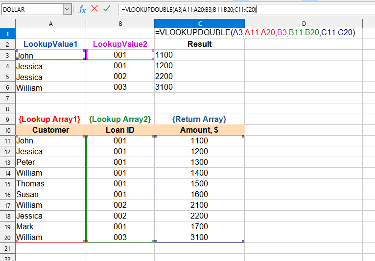
The VLOOKUPDOUBLE() function is easy to use. You just need to specify 2 separate search ranges, 2 values for comparison, and the column from which the associated values will be returned, and Excel (Calc) will automatically find and return the required result for two matches:
=VLOOKUPDOUBLE(LookupValue1; Lookup Array1; LookupValue2; Lookup Array2; Return Array)
We will have the following result:


In this example, the following values are used:
You can use the function VLOOKUPDOUBLE() by installing the extension YLC Utilities.
After that, this function will be available in all files that will be opened in Excel (LibreOffice Calc).