Join Tables (VLOOKUP)

What is VLOOKUP

The built-in function VLOOKUP is one of the most powerful functions in Excel. It belongs to the three most popular in Excel — after SUM and AVERAGE. Her task is to find the desired value in the data table and display it in the specified cell.

The function syntax includes a lookup value (what you're looking for), a table with one or more columns (where to look), a column index number (from which column to return data), and a lookup type (an additional argument that lets you choose an approximate or exact result).

The VLOOKUP function is commonly used for financial analysis, data management, and working with databases. Using this feature, users can quickly and easily find information in a large data set, which can save time and improve accuracy.

The VLOOKUP function looks for values vertically, that is, among rows (this is indicated by the first letter V - Vertical). In Excel, there is also a similar function HLOOKUP, which has a similar functionality, but makes a horizontal (H - Horizontal) search by columns.

An example of a problem

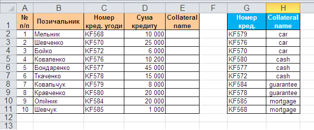
Suppose we have two tables with data - loan table and collateral table :

We need to automatically insert collateral into the loan table, based on the agreement number, for further reporting.

Solution

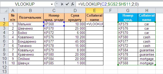
In Excel in the standard set of functions in the category Lookup and reference is a function VLOOKUP . This function looks for the specified value (in our example, the agreement number) in the leftmost column of the specified table (security table) moving from top to bottom and, finding them, displays the value of the adjacent cell (type of credit security). Schematically, the operation of the function looks like this:

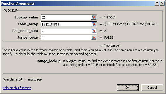
So, let's use the function VLOOKUP . Select the cell where it will be entered ( E2 ) and open the formula wizard (menu Insert - Function ). In the category (Lookup and Reference) find the function VLOOKUP and press OK . A window will appear for entering function arguments:

Fill them in one by one:

• Lookup Value - the agreement number, which the function will look for in the far left column of the provisioning table. In our case - the agreement number "KF568" from the cell C2 .
• Table Array - the table from which we will get the required values is our supply table. We'll use a range for the reference $G$2:$H$11 (the range is fixed with a dollar sign ($) , so that it does not move to the bottom when copying the formula).
• Column index number - the serial number (not a letter!) of the column in the provision table, from which we will take the name of the provision. The first column of the provision table has the sequence number 1, so we need to take the type of provision from the second column (number 2).
• Range Lookup - we can enter only two values in this field: TRUE or FALSE:
  
  1) If we enter a value 0 or FALSE , then this actually means that only search is allowed with an exact match , that is, if the function does not find the agreement number in the provisioning table (if it does not exist), then an error will be displayed #N/A (no data).
  
  2) If we enter a value 1 or TRUE , this will mean that it is allowed to search not only exact, but also approximate coincidence . In most cases, such an approximate substitution can cause a false result when VLOOKUP will substitute the values of other agreements. So, you should use approximate search only for numeric values (pre-sorted in ascending order).

It remains to press OK and copy the entered function across the entire column.

Disadvantages of the VLOOKUP function

The main disadvantage is that the search for the desired value can only take place in the first column of the given range, and the function can return the desired value only from the columns to the right.

The second disadvantage of VLOOKUP is that the function stops working if you remove or add a column to the lookup table. An inserted or deleted element will change the result of the formula because the function syntax requires that you specify the entire range and the specific column number from which you want to extract data.

Also, the VLOOKUP function has a lookup length limit of 255 characters, otherwise the #VALUE error will be returned!

Problems when working with the function

Function VLOOKUP returns an error (#N/A) if:

1. Exact search is allowed (argument Range Lookup=0) and the searched value is not in the table (Table) .
2. Approximate search allowed (Range Lookup=1), but in the table (Table) , in which we search for values, the names are not sorted in ascending order.
3. The format of the cell from which we take the transaction number (for example, C2 in our case) and the cell format of the first column (G2:G11) tables are different (for example, numeric and text). This situation is particularly typical when numerical codes are used instead of textual names (account numbers, identification codes, dates, etc.). In this case, you can use functions VALUE and TEXT to convert data formats. It looks like this:
   =VLOOKUP(TEXT(C2);$G$2:$H$11;0) .
4. The function does not find a value because the code contains spaces and invisible non-printing characters (tape feeds, etc.). In this case, you can use the text function (TRIM) and (CLEAN) to remove them:
   =VLOOKUP(TRIM(CLEAN(C2));$G$2:$H$11;0) .

Error suppression

To suppress the error message (#N/A) , when the function cannot find an exact match, you can use the function IFERROR . This function checks if an error (#N/A) is the result of work VLOOKUP , and if so, outputs an empty tape ( "" ) or zero, if not - the result of the work VLOOKUP .

Related Articles:

• Improved function VLOOKUP (VLOOKUP2)
• VLOOKUP for combination according to two conditions (VLOOKUP3)
• Quick merge of large tables (VLOOKUP2D)