Linked drop-down lists

Description

In Excel you can quickly and easily create a dropdown list , but have you ever tried creating a dependent dropdown list? There are several ways to create such a list, so let's take a look at them.

Method 1. INDIRECT function

This technique is based on the application of the INDIRECT function, which can do one simple thing - convert the contents of any specified cell into a range address that Excel understands. That is, if the cell contains the text " А1 ", then the function will give a reference to the cell as a result А1 . If the cell contains the word " Auto ", then the function will output a reference to the named range with the name Auto etc.

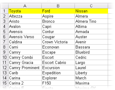
Take, for example, this list of car models Toyota, Ford and Nissan :

Select the entire list of Toyota models (from cell А2 and down to the end of the list) and give this range a name Toyota in the menu Insert - Name - Assign (Insert - Name - Define) . Then we will repeat the same with the lists Ford and Nissan , specifying the names of the ranges accordingly Ford and Nissan .

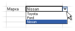
Now let's create the first drop-down list for choosing a car brand. Select an empty cell and open the menu Data - Check (Data - Validation) , then from the drop-down list Data type select an option List and in the field Source - highlight cells with brand names (yellow cells in our example). After clicking on ОК the first drop-down list is ready:

Now let's create a second drop-down list, which will display the models of the brand selected in the first list. Just like in the previous case, select an empty cell and open the menu Data - Check - further List . In the field Source you will need to enter the following formula:

=INDIRECT(F3)

Where:

• F3 - the address of the cell with the first drop-down list - replace it with yours.

All. After clicking on OK the contents of the second list will be selected by the name of the range selected in the first list.

Cons of this method:

• Dynamic ranges specified by OFFSET type formulas cannot act as secondary (dependent) ranges. You can use them for the primary (independent) list, but the secondary list must be defined rigidly, without formulas.
• The secondary range names must match the primary dropdown list items. That is, if it contains text with gaps, they will have to be replaced with underlines, etc.
• You need to manually create many named ranges.

Method 2. Match list (OFFSET and MATCH)

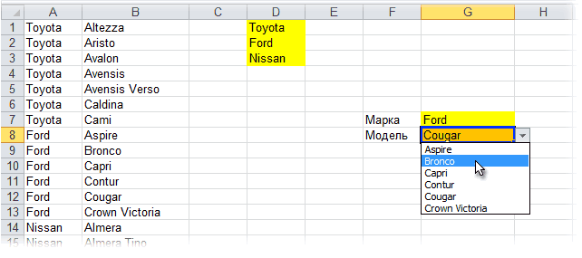
This method requires a sorted list of make-model matches of the following type:

To create a primary drop-down list of brands, you can use the usual method described above, that is:

• Give the name of the range D1:D3 (eg Brands )
• Select on the tab Data (Data) team Data verification (Data validation)
• Select a check option from the drop-down list List (List) and specify as quality Sources (Source) = Brands or simply select cells D1:D3 (if they are on the same sheet as the list).

But for a dependent list of models, you will have to create a named range with the function OFFSET, which will dynamically refer only to cells of models of a certain brand. For this:

• Press Ctrl + F3 or use the button Name manager (Name manager) on the tab Formulas (Formulas) . In versions before 2003, this was a menu command Insert - Name - Assign (Insert - Name - Define)
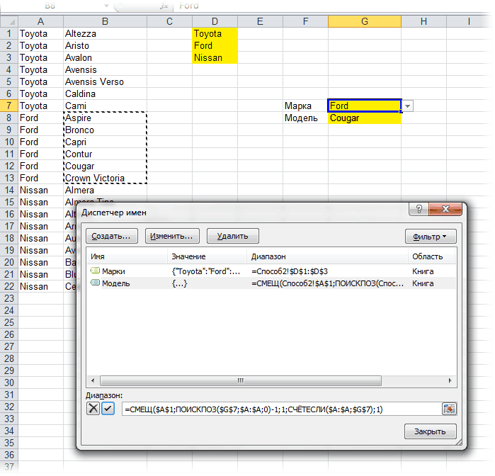
• Create a new named range with any name (eg Models ) and in the field Link (Reference) in the lower part of the window, manually enter the following formula:

=OFFSET( $A$1 ; MATCH($G$7;$A:$A;0)-1 ; 1 ; COUNTIF($A:$A;$G$7) ; 1 )

The function OFFSET is able to issue a reference to a range of the desired size, shifted relative to the initial cell by the given number of rows and columns. In a more understandable version, the syntax of this function is as follows:

=OFFSET( start_cell ; shift_down ; shift_right ; range_size_in_rows ; range_size_in_columns )

So:

• start_cell - we take the first cell of our list, i.e A1 ;
• shift_down - we count the MATCH function, which, simply put, outputs the serial number of the cell with the selected brand (G7) in the given range (columns AND );
• shift_right =1 , so we want to refer to the models in the adjacent column ( IN );
• range_size_in_rows - we calculate using the COUNTIF function, which is able to count the number of occurrences in the list (column A) of the values we need - car brands ( G7 );
• range_size_in_columns =1 , so we need one column with models.

The result should be something like this:

It remains to add a drop-down list based on the created formula to the cell G8 . For this:

• Select a cell G8
• Select on the tab Data (Data) team Data verification (Data validation) or in the menu Data - Check (Data - Validation)
• Select the check option from the drop-down list List (List) and enter as Sources (Source) sign is equal to the name of our range, i.e = Models .

Related Articles:

• A drop-down list in a cell
• A hint when filling in data in a cell