Creating Pivot Tables (PivotTables)

Description

Summary table (Pivot Table) is a powerful data calculation, summarization, and analysis tool that lets you see comparisons, patterns, and trends in your data.

Imagine that you need to make a short analytical report for decision-making from a large table that contains a lot of different information. Suppose you have data that displays information on the Bank's loan portfolio, where detailed information on each borrower is recorded.

An example of a problem

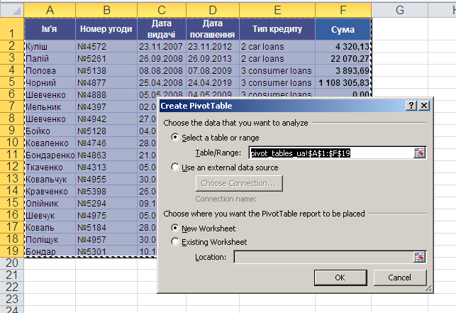
Let's assume that the following table is loaded from the database into Excel to analyze the loan portfolio:

In it, each individual line contains complete information about one credit agreement:

• name of the borrower;
• agreement number;
• date of issuance and repayment date of the loan;
• type of loan;
• loan amount

Naturally, if sales managers know their business and work hard, then every day several tens of lines will be added to this table, and by the end of, for example, a year or at least a quarter, the size of the table will become monstrous.

However, even greater horror will cause you the need to create reports based on this data. How many loans were issued each month? What is the size of the loan portfolio in terms of lending by quantity and amount? Top ten borrowers? etc.

Answers to all questions can be obtained more easily than you think. About three minutes. With one of the most amazing tools Microsoft Excel — Summary tables .

Let's go...

Data preparation

Consider the following data preparation tips before creating PivotTables:

• use clean tabular data for best results;
• place data in columns, not rows;
• ensure that all columns have headers with one line of unique non-empty captions for each column. Avoid duplicate header rows or merged cells;
• format the data as "smart table Excel" (click anywhere on your data, then select "Insert" - "Table" ( Insert - Table ) in the ribbon menu (ribbon);
• if you have complex or nested data (like a crosstab), use Power Query to convert them (for example, you can use a macro to cancel data summary ) so that they are organized in columns with a single header row.

Creating a Pivot Table

Select our entire data table and click on the menu Insert - Summary table ( Insert - PivotTable ).

This dialog box will appear, in which we can choose where to place our pivot table and adjust the data range.

By default, Excel chooses to place the pivot table on a new sheet (New Worksheet) , but we can, if necessary, manually select the current or any other sheet of the book (Existing Worksheet) . It is better to choose a new sheet for this - then there is no risk that the summary table will "overlap" with the original list and we will get a bunch of cyclic links. Press the button OK and we move on to the most interesting part - the stage of constructing our report.

Working with the layout

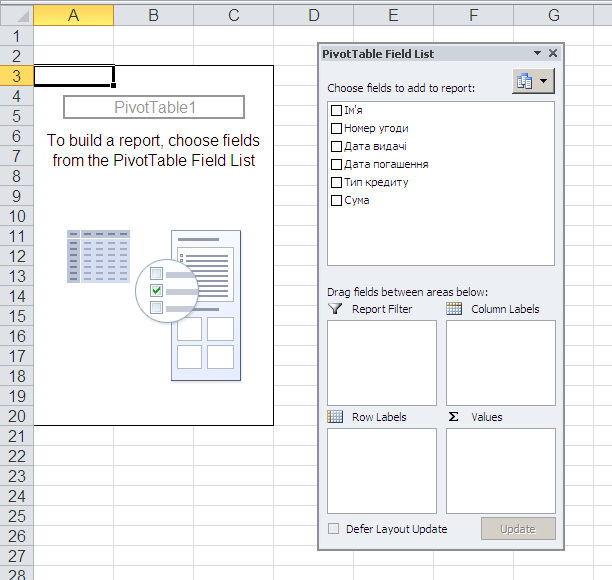
What you will see after pressing the button OK called a layout (layout) summary table:

It is easy to work with it - you need to drag the names of the columns (fields) from the window with the mouse List of fields of the summary table (PivotTable Field List) in the region:

• rows (Row Labels);
• columns (Column Labels);
• filters (Report Filter);
• layout data (Values).

The only caveat is to do it more precisely, don't miss! Let's go...

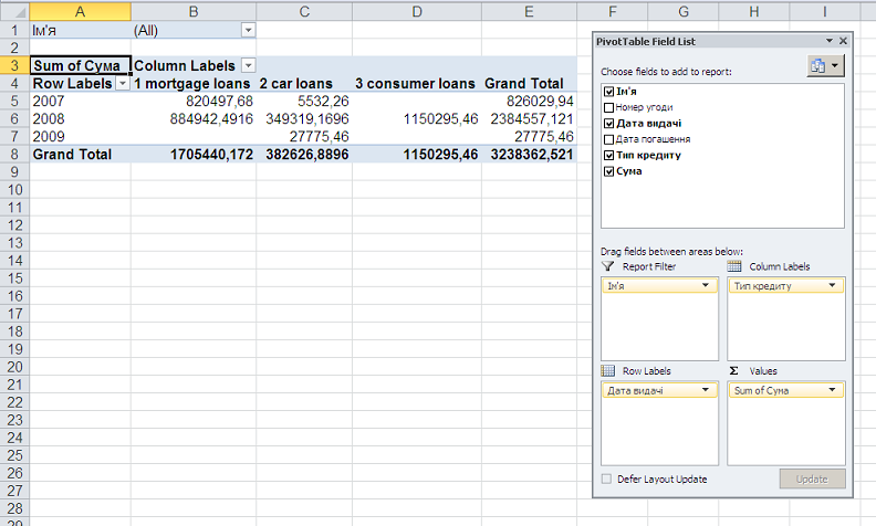
In the process of dragging, the consolidated table will begin to change its appearance before your eyes, displaying the data you need. After crossing all the four fields we need from the list, you should get an almost ready report. It remains only to format it well.

Formatting of the Pivot Table

Select the formatting of the summary table in the menu PivotTables Tools - Design :

But we get the following look:

It's not that complicated, is it?

Disadvantages

The only drawback of summary tables is the lack of automatic updating (recalculation) when the data in the original list changes. To perform such a calculation, it is necessary to click on the summary table with the right mouse button and select the command in the context menu Update (Refresh) .

Related Articles:

• Unpivottables (Unpivot)
• PowerPivot - an application for expanding the capabilities of Pivot Tables